2 alternatives to Excel VLookUp
VLookUp is a powerful and useful function in Excel. It allows you to look up a value in a list and return any column from the look-up column, left. If your first column had employee ID and your seventh column had ZIP code, VLookUp could find the ZIP code for a whole list of employee IDs. The formula would look similar to this: =VLOOKUP(A1,Employee_Table, 7,0), where A1 contains the employee ID and all employee records are stored in a named range called Employee_Table.
But what if your look-up column isn’t the first one? Your work around might be to copy the look-up column to a newly inserted first column. However, there are two better ways. Meet Index-Match and LookUp. These two methods even allow you to look up a value across a row and return a value from a column.
Index-Match
Technically, Index-Match is more efficient than a VLookUp because it doesn’t have to process the entire table. It only has to process the column or row that has your look-up value and the column or row that has your result. The bigger your data gets, the more this might be a worthwhile consideration. The Index function requires you first to tell it the range of cells that will contain your desired result. Then, it wants to know how many cells down your range to go to find what you want based on a look-up value you provide. So in this example, if we looked up the course code LW102 (our look-up value in A1) from D3:D5 (look-up range) and wanted to return the course name, a plain Index formula would look like this =INDEX(A3:A5,2).
But how would it know that it’s in the second row down? Without a Match function, it wouldn’t. Match returns the position in the range 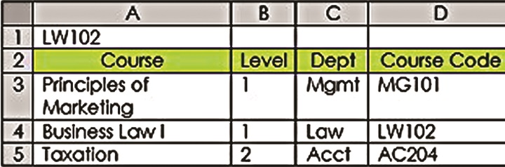 corresponding to the look-up value. So =MATCH (A1,D3:D5,0) would return 2. Adding the zero on the end means find the value exactly or return #N/A. Putting them together as =INDEX(A3:A5,MATCH (A1,D3:D5,0 )) translates to: in the range A3:A5, return the value corresponding to a range position equal to the place where you find my look-up value (LW102) in D3:D5. Unlike most look-up functions, the Index-Match combo starts with the range where you’ll find the answer, followed by where you’ll find the look-up value. With VLookUp, HLookUp and LookUp you begin with where you’ll find your look-up value, then the location of the result.
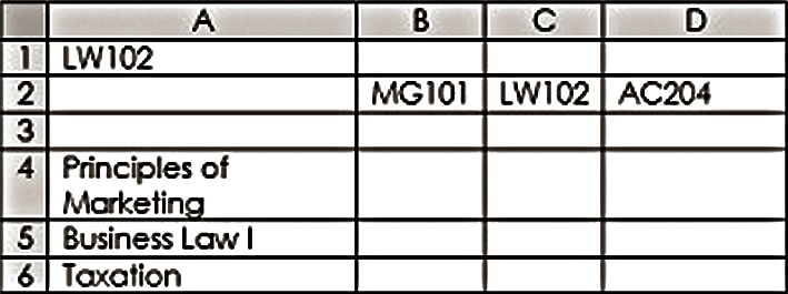
You could also use Index/Match to return a value based on a look-up in another range entirely. So your Course Codes could be listed across a row in another table, but because it would find it in the second cell in the range, the value 2 would be returned to find the second cell in the result range, even if that were down a column. That might look like this=INDEX(A4:A6,MATCH(A1,B2:D2,0)), given the second data layout.
LookUp
The LookUp function is even easier because it does not require a Match function, only the look-up value, look-up range and result range. In the first data example, the formula would be =LOOKUP(A1,D3:D5,A3:A5). In the second example, it would have been written =LOOKUP(A1,B2:D2,A4:A6). You might be asking, “Why would I even go through all the trouble of Index-Match if LookUp is this easy?” The advantage of Index-Match is that you can specify “exact” as a match type. This is required if your list is not sorted in ascending order.